
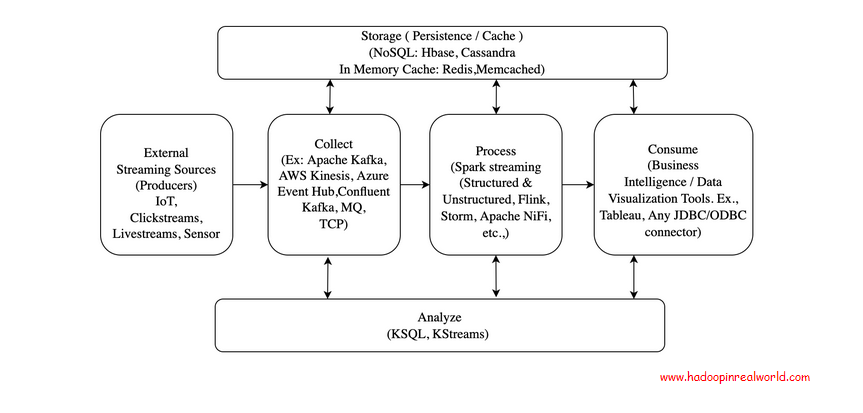
Building Big Data Streaming Pipelines – architecture, concepts and tool choices
May 4, 2020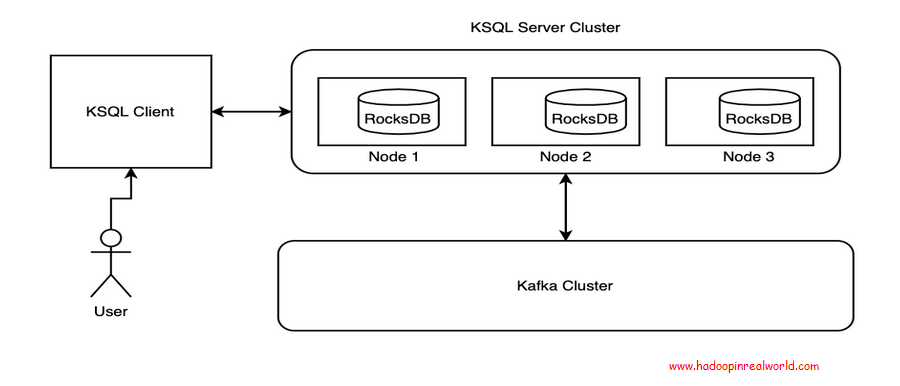
Building Stream Processing Applications using KSQL
June 1, 2020
Those in the industry know that one of the best techniques for catching malware using Machine Learning (ML) is only possible with distributed computing. Before showing you the math of why it requires distributed computing, let me tell you what this technique is and why it is the best one.
The Best Technique In The Business
This technique, to be named in a moment, is one of the best feature extraction techniques because
- It works on every type of sample
- It does not rely on hand-made features – it is automatic.
If you’re familiar with ML, you might wonder, why would not relying on hand-made features make a difference?
Malware detection is an adversarial domain, where hackers are constantly finding ways to evade malware detectors. They can “stuff” malware with benign features, hide malware inside benign files (“trojaning”) and have a myriad of other ways of avoiding being detected. In particular, hand-designed features are too easy for hackers to reverse-engineer and then evade.
So what is this technique? It is featurizing samples via N-grams of their byte code sequence. This technique is pretty much the industry standard backbone for a ML malware detector. Before I show you how to implement it in code, let’s understand how it works and look at the math to see why you need distributed computing to execute it.
How It Works
Take a sample file, say the python 3.7.7 installer, available at https://www.python.org/ftp/python/3.7.7/python-3.7.7-amd64.exe
We can use the xxd tool in bash to take a peek at the first few bytes of this file
xxd -p python-3.7.7-amd64.exe | head -n 1
The output is a truncated sequence of bytes:
4d5a90000300000004000000ffff0000b800000000000000400000000000
There are a lot more bytes where those came from. The file is approximately 25.5mb. Can you tell how many bytes that is?
Let’s do a quick calculation. 1mb is 1024 kb and 1kb is 1024 bytes, so the number of bytes is approximately
25.5 x 1024 x 1024 = 26,738,688
In other words a typical file is a sequence of about 27 million bytes. The technique calls for “N-Grams” on this sequence of bytes, so let’s understand what that means.
Generally speaking, an “N-Gram” is a sequence of “N” consecutive “Grams”. The “N” is a placeholder for a number. For example, there are “1-Grams”, “2-Grams”, “3-Grams”, and so on.
The “Gram” in our context is a byte. So in our sample file,
-   The 1-Grams are “4d”, “5a”, “90”, “00”, “00”,...
-   The 2-Grams are “4d 5a”, “5a 90”, “90 00”, “00 00”,...
-   The 3-Grams are “4d 5a 90”, “5a 90 00”,...
-   etc.
These N-Grams hold in them local statistical information about the sample being examined. For that reason ML classifiers are able to leverage these N-Grams to yield precise predictions on whether a file is malicious or benign before it even runs!
Enjoying the post? Check out more projects at our Spark Developer In Real World course!
The Computational Challenge
Now in order to feed the N-Grams into a classifier, several steps are in order, such as selecting the optimal N in N-Grams, selecting the topmost statistically significant N-Grams, and producing feature vectors for the samples from the counts of these selected “best” N-Grams. For our discussion, the most important problem is counting the N-Grams in all the files. This problem is a computational Everest.
Let’s do the math at a high level. We want a dictionary of counts for each N-Gram over all of the files. A cybersecurity enterprise will have literally millions of samples in their dataset. Each sample is typically several million bytes. This means it will have several million N-Grams. Since there are 256 bytes, there are 256^N types of N-Grams. This means that the dictionary will have up to 256^N keys. To get a sense of the magnitude, note that
– For N=2: 256^N = 65,536,
– For N=3: 256^N = ~16.7 million,
– For N=4: 256^N = ~4 billion
The time and space requirements are gigantic. Fortunately, it is possible (and necessary) to distribute the task, which is where Hadoop and Spark come into play.
Take a moment to think this problem through in terms of Map-Reduce. When ready, read on.
Map-Reduce Solution
In a Map-Reduce paradigm, our mappers will take groups of files, and for each file, produce a dictionary of N-Gram counts. Our reducers will add these dictionaries. Our final output will be the sum of all these dictionaries, i.e., all N-Gram counts. So now let’s see how to actually code this problem in PySpark.
PySpark Implementation
For the remainder, the code and dataset are available at https://github.com/hadoopinrealworld/how-to-catch-malware-using-spark. Note that the dataset contains live samples so only run it in a safe environment, such as a Virtual Machine (VM).
- Begin by cloning the data:
!git clone https://github.com/emmanueltsukerman/how-to-catch-malware-using-spark.git
- Unzip and create directories for the data. The password is “infected”. Again, only do this in a safe environment or skip the malicious samples.
!7z e "/content/how-to-catch-malware-using-spark/PE Samples Dataset/Benign PE Samples 1.7z" -o"/content/benign"

!7z e "/content/how-to-catch-malware-using-spark/PE Samples Dataset/Benign PE Samples 2.7z" -o"/content/benign"

!7z e "/content/how-to-catch-malware-using-spark/PE Samples Dataset/Benign PE Samples 3.7z" -o"/content/benign"

!7z e "/content/how-to-catch-malware-using-spark/PE Samples Dataset/Benign PE Samples 4.7z" -o"/content/benign"

!7z e "/content/how-to-catch-malware-using-spark/PE Samples Dataset/Benign PE Samples 5.7z" -o"/content/benign"

!7z e "/content/how-to-catch-malware-using-spark/PE Samples Dataset/Benign PE Samples 6.7z" -o"/content/benign"

# Use the industry standard password for malware-containing zip files

!7z e "/content/how-to-catch-malware-using-spark/PE Samples Dataset/Malicious PE Samples 1.7z" -o"/content/malicious" -p'infected'

!7z e "/content/how-to-catch-malware-using-spark/PE Samples Dataset/Malicious PE Samples 2.7z" -o"/content/malicious" -p'infected'

!rm -r "/content/benign/Benign PE Samples 1"

!rm -r "/content/benign/Benign PE Samples 2"

!rm -r "/content/benign/Benign PE Samples 3"

!rm -r "/content/benign/Benign PE Samples 4"

!rm -r "/content/benign/Benign PE Samples 5"

!rm -r "/content/benign/Benign PE Samples 6"

!rm -r "/content/benign/Malicious PE Samples 1"

!rm -r "/content/benign/Malicious PE Samples 2"
- Install PySpark if you don’t have it already
!apt-get install openjdk-8-jdk-headless

import os

os.environ["JAVA_HOME"] = "/usr/lib/jvm/java-8-openjdk-amd64"

!pip install pyspark
Like what you are reading? You would like our free live webinars too. Sign up and get notified when we host webinars =>
- Initialize your spark session
from pyspark.sql import SparkSession


# Build the SparkSession

spark = SparkSession.builder \

   .master("local") \

   .appName("Malware Detector") \

   .config("spark.executor.memory", "1gb") \

   .getOrCreate()


sc = spark.sparkContext
- We are going to create a pipeline to count the N-Grams and then featurize these.
We will end up with the most frequent `NUM_NGRAMS=100` N-grams, which are also generally the most statistically significant ones. We will then train a classifier using these as features.
from pyspark.ml.feature import NGram, CountVectorizer, VectorAssembler

from pyspark.ml import Pipeline

from pyspark.ml.classification import LogisticRegression


NUM_NGRAMS = 100

def build_ngrams(inputCol="byte_content", N=2):
    ngrams = [

        NGram(n=N, inputCol="byte_content", outputCol="{0}_grams".format(N))

    ]

    vectorizers = [

        CountVectorizer(inputCol="{0}_grams".format(N),

            outputCol="{0}_counts".format(N),

            vocabSize = NUM_NGRAMS)

    ]

    assembler = [VectorAssembler(

        inputCols=["{0}_counts".format(N)],

        outputCol="features"

    )]

    lr = [LogisticRegression(maxIter=100 )]

    return Pipeline(stages=ngrams + vectorizers + assembler+lr)
- Read in the binary files into RDDs:
benign_rdd = sc.binaryFiles("benign")

malicious_rdd = sc.binaryFiles("malicious")
Let’s take a peek at what we have so far:
benign_rdd.first()

('file:/content/benign/ImagingDevices.exe', b'MZ\x90\x00\x03\x00\x00\x00\x04\x00\x00\x00\xff\...)
You are seeing the name of the sample and its byte sequence.
- We will convert these RDDs to dataframes for ease of use. We will also limit the number of bytes we take from each sample to `BYTES_UPPER_LIMIT = 5000` to make the computation easier for this tutorial.
from collections import namedtuple

BYTES_UPPER_LIMIT = 5000

Sample = namedtuple("Sample", ["file_name", "byte_content"])


benign_df = benign_rdd.map(lambda rec: Sample(rec[0], [str(x) for x in bytes(rec[1])][0:BYTES_UPPER_LIMIT])).toDF()

malicious_df = malicious_rdd.map(lambda rec: Sample(rec[0], [str(x) for x in bytes(rec[1])][0:BYTES_UPPER_LIMIT])).toDF()
- Label the benign samples with 0 and the malicious sample with 1
from pyspark.sql.functions import lit

benign_df = benign_df.withColumn("label",lit(0))

malicious_df = malicious_df.withColumn("label",lit(1))
The dataframes now look like so:
benign_df.show(5)

malicious_df.show(5)
- Combine the dataframes into one, as we will run the pipeline on all files at once.
df = benign_df.unionAll(malicious_df)
- Create a training-testing split
df_train, df_test = df.randomSplit([0.8,0.2])
- Fit the pipeline onto the data.
trained_vectorizer_pipeline = build_ngrams().fit(df) (this line should be erased)

trained_vectorizer_pipeline = build_ngrams().fit(df_train)
Note that in step 5, we have specified in our CountVectorizer to build a vocabulary that only considers the top NUM_NGRAMS = 100 N-Grams ordered by term frequency across the corpus. More advanced implementations, such as mutual information-based feature extraction or Random Forest feature selection can be used. However, despite the apparent simplicity of the frequency approach, it has been shown to be the most successful method for selecting N-Grams, both in the literature (see, e.g., “An Investigation of Byte N-Gram Features for Malware Classification”, Raff et al.) and in industry.
- Featurize and classify the testing dataset.
df_pred = trained_vectorizer_pipeline.transform(df_test)
See that we have featurized our samples
df_pred.show(5)
- Finally, we can calculate the accuracy of our classifer on the testing data
accuracy = df_pred.filter(df_pred.label == df_pred.prediction).count() / float(df_pred.count())
Our accuracy is
0.9759036144578314
which is spectacular for a data set of this size!
We have successfully featurized our samples and trained a prototype classifier that will be able to tell us when a new file is malware, safeguarding us and our data from harm.
Congratulations!
Like what you are reading? You would like our free live webinars too. Sign up and get notified when we host webinars =>